How to use the latest National Land Cover Database 2011 (NLCD 2011) in CALMET
The National Land Cover Database 2011 (NLCD 2011) provides the land cover classification of the United States territory at a spatial resolution of 30m. It is based on the Landsat 2011 satellite data and is the latest of the series started with NLCD2001.
The land cover information is a necessary input to the meteorological preprocessor CALMET, part of the CALPUFF 7.0 modeling system. The land cover information is input via the GEO.DAT file and it can be prepared by processing a number of data sources using the CTGPROC program distributed with CALPUFF.
The input formats available in CTGPROC 7.0 are:
-------------
Subgroup (0b)
-------------

     The following NDBF Land Use Data Files are processed.
     Enter NDBF lines identifying the file name for each,
     followed by a group terminator.  The type of data base
     for each file is designated by the assignment name:

     (CTG)     designates USGS CTG (compressed)
     (GEN)     designates Generic (no USGS translation is done)
     (NZGEN)   designates New Zealand Generic
     (GLAZNA)  designates USGS Global (Lambert Azimuthal) for North America
     (GLAZSA)  designates USGS Global (Lambert Azimuthal) for South America
     (GLAZEU)  designates USGS Global (Lambert Azimuthal) for Eurasia - Europe
     (GLAZAS)  designates USGS Global (Lambert Azimuthal) for Eurasia - Asia
     (GLAZAF)  designates USGS Global (Lambert Azimuthal) for Africa
     (GLAZAP)  designates USGS Global (Lambert Azimuthal) for Australia-Pacific
     (NLCD92)  designates National Land Cover Dataset 1992 Flat
     (NLCDTF)  designates National Land Cover Dataset 1992 GeoTIFF
     (NLCD01)  designates National Land Cover Dataset 2001 GeoTIFF
     (GLC2K)   designates Global Land Cover 2000 GeoTIFF
     (UMDGLC)  designates Univ. of Maryland Global Land Cover GeoTIFF
     (MODIS)   designates Boston Univ. Modis Global Land Cover
Among these, only NLCD* ones are providing information at high resolution (30m). This is a need when the CALMET grid size is small, since the other land use data files have a much coarser resolution.
Unfortunately the more recent NLCD2006 and NLCD2011 cannot be used because they are in BigTIFF format (the evolution of the TIFF format to support files larger than 4 GB).
Since the land use is changing significantly in time, for example in areas of new urbanization, it can be importan to use these more recent data.
The following procedure outline gives some hints on how to do that. As an example a domain in New York is defined (KML file).

Using Linux or OS X is recommended so that the Perl module Geo::Proj4 can be used.
The procedure also uses ImageMagick's convert script.
Download the NLCD2011 database.
Save the following Perl code in a file, for example script1.pl:
use strict;
use Geo::Proj4;

# Change window as needed
my $ul = [-74.1,40.85];
my $lr = [-73.99,40.65];

# No changes below
my $from  = Geo::Proj4->new("+proj=latlong +datum=NAD83");
my $to    = Geo::Proj4->new("+proj=aea +lat_1=29.5 +lat_2=45.5 +lat_0=23 +lon_0=-96 +x_0=0 +y_0=0
    +ellps=GRS80 +datum=NAD83 +units=m +no_defs");

my $ul_p = $from->transform($to,$ul);
my $lr_p = $from->transform($to,$lr);
print "gdal_translate -of GTiff -co \"BIGTIFF=NO\"";
print "-projwin $ul_p->[0] $ul_p->[1] $lr_p->[0] $lr_p->[1] input_file output_file \n";
This program converts the coordinates of your Lon/Lat window into the Albers Conical Equal Area projection of the NLCD database and prints (on one line) in output a string that we use as template for the input command we need to extract from the NLCD2011 database the tile of interest in GeoTIFF format:
roberto@vespaiolo:~/tmp$ perl script1.pl
 gdal_translate -of GTiff -co "BIGTIFF=NO"
-projwin 1815127.86523829 2192268.61342957 1829223.21737201 2172573.74776145
input_file output_file
We change input_file to the path and filename of the file nlcd_2011_landcover_2011_edition_2014_10_10.img we find in the database downloaded and we choose a name for the output, for example tile.tif. If all works the message we obtain upon execution is:
Input file size is 161190, 104424
Computed -srcwin 143605 37257 470 656 from projected window.
0...10...20...30...40...50...60...70...80...90...100 - done.
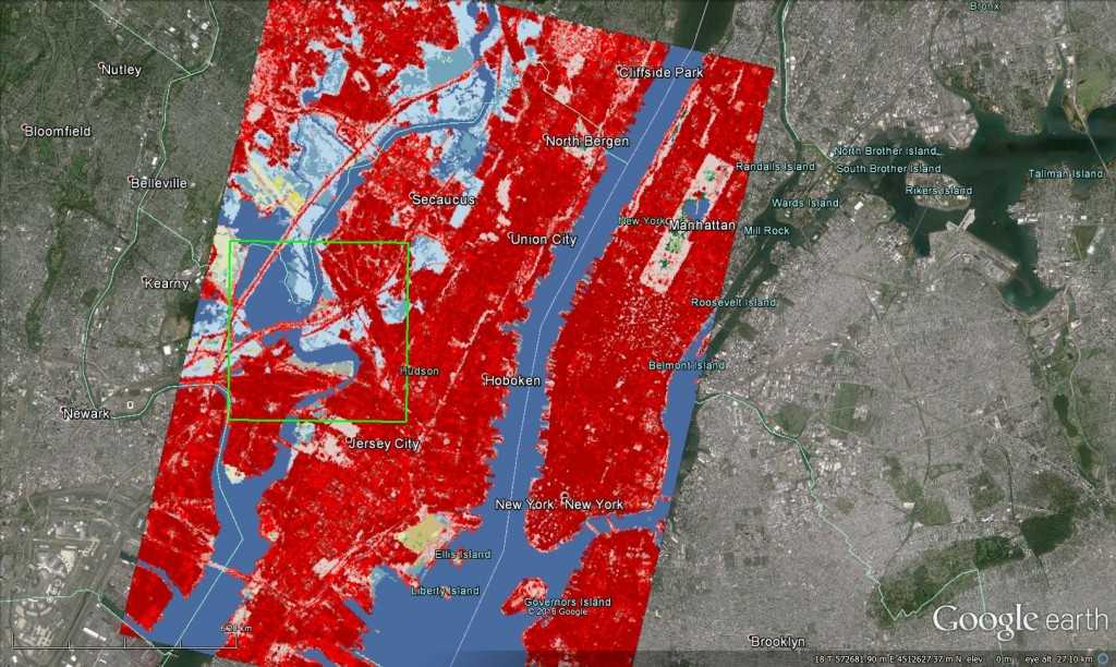
And this is the tile imported in Google Earth:

We then run the convert program on the Tiff output file, to extract the RGB values that associate each pixel to the land cover value.
roberto@vespaiolo:~/tmp$ convert tile.tif tile.txt
The output messages may contain some warnings about unknown private tags that shouldn't be harmful, for example:
convert.im6: Unknown field with tag 33550 (0x830e) encountered. `TIFFReadDirectory' @ warning/tiff.c/TIFFWarnings/768.[/code]
The tile.txt generated file contains tha RGB for each pixel as a list:
# ImageMagick pixel enumeration: 470,656,255,srgb
0,0: (221,201,201)  #DDC9C9  srgb(221,201,201)
1,0: (216,147,130)  #D89382  srgb(216,147,130)
2,0: (237,  0,  0)  #ED0000  srgb(237,0,0)
3,0: (216,147,130)  #D89382  srgb(216,147,130)
4,0: (216,147,130)  #D89382  srgb(216,147,130)
5,0: (237,  0,  0)  #ED0000  srgb(237,0,0)
6,0: (170,  0,  0)  #AA0000  srgb(170,0,0)
7,0: (237,  0,  0)  #ED0000  srgb(237,0,0)
8,0: (237,  0,  0)  #ED0000  srgb(237,0,0)
...
We need to extract the Origin of the tile and the pixel size (that we already know is 30m..) so that we will be able to transform the pixel indices to georaphical coordinates:
roberto@vespaiolo:~/tmp$ gdalinfo tile.tif | perl -ne 'print if /Origin/../Pixel/'
Origin = (1815105.000000000000000,2192295.000000000000000)
Pixel Size = (30.000000000000000,-30.000000000000000)
And we need to extract the color table:
roberto@vespaiolo:~/tmp$ gdalinfo tile.tif | perl -ne 'print if /Color Table/../DUMMY/' > tile.clt
The color table has one record for each RGB, and non-zero values correspond to NLCD Land cover classes:
  Color Table (RGB with 256 entries)
    0: 0,0,0,255
    1: 0,249,0,255
    2: 0,0,0,255
    3: 0,0,0,255
    4: 0,0,0,255
    5: 0,0,0,255
    6: 0,0,0,255
    7: 0,0,0,255
    8: 0,0,0,255
    9: 0,0,0,255
   10: 0,0,0,255
   11: 71,107,160,255
   12: 209,221,249,255
   13: 0,0,0,255
   14: 0,0,0,255
   15: 0,0,0,255
...
You will then need to write some script that reads the tile.txt file and for each pixel converts its I,J indexes in geographical coordinates and its RGB in NLCD2011 Land Cover category first and then to CALMET default USGS categories. With Perl it is useful to use the already seen Geo::Proj4 module.
The NLCD categories are defined for example in CTGPROC:
From ctgproc.for, line 586
      data nlcd01/10*0,
     1            52,91,8*0,
     2            30,11,11,13,6*0,
     3            74,72,8*0,
     4            41,42,43,7*0,
     5            32,32,8*0,
     6            10*0,
     7            31,82,82,82,6*0,
     8            2*21,7*0,
     9            5*61,5*62
This is the association from NLCD categories to intermediate categories:
    11 =>   52, #   Open water => Lakes
    12 =>   91, #   Perennial Ice/Snow => Perennial Snowfields
    21 =>   30, #   Developed - Open Space => Rangeland
    22 =>   11, #   Developed - Low intensity => Residential
    23 =>   11, #   Developed - Medium intensity => Residential
    24 =>   13, #   Developed - High intensity => Industrial
    31 =>   74, #   Barren Land (Rock/Sand/Clay) => Bare Exposed Rock
    41 =>   41, #   Deciduous Forest => Deciduous Forest Land
    42 =>   42, #   Evergreen Forest => Evergreen Forest Land
    43 =>   43, #   Mixed Forest => Mixed Forest Land
    51 =>   32, #   Dwarf Scrub => Shrub and Brush Rangeland
    52 =>   32, #   Shrub/Scrub => Shrub and Brush Rangeland
    71 =>   31, #   Grassland/Herbaceous => Herbaceous Rangeland
    72 =>   82, #   Sedge/Herbaceous => Herbaceous Tundra
    73 =>   82, #   Lichens => Herbaceous Tundra
    74 =>   82, #   Moss => Herbaceous Tundra
    81 =>   21, #   Pasture/Hay => Cropland and Pasture
    82 =>   21, #   Cultivated Crops => Cropland and Pasture
    90 =>   61, #   Woody wetlands => Forested Wetland
    95 =>   61 ,#   Emergent Herbaceous Wetlands => Forested Wetland
And then to USGS categories:
           LAND USE PROPERTIES AND OUTPUT MAP (NINCAT entries)
           ---------------------------------------------------

     Input                                 Soil   Anthropogenic Leaf   Output
    Category    z0     Albedo    Bowen   Heat Flux  Heat Flux   Area  Category
       ID       (m)   (0 to 1)   Ratio   Parameter  (W/m**2)   Index     ID
     ------   ------   ------    ------  ---------  --------   ------  ------

! X =    11,       1,    0.18,     1.5,     0.25,        0,      0.2,     10!  !END!
! X =    12,       1,    0.18,     1.5,     0.25,        0,      0.2,     10!  !END!
! X =    13,       1,    0.18,     1.5,     0.25,        0,      0.2,     10!  !END!
! X =    14,       1,    0.18,     1.5,     0.25,        0,      0.2,     10!  !END!
! X =    15,       1,    0.18,     1.5,     0.25,        0,      0.2,     10!  !END!
! X =    16,       1,    0.18,     1.5,     0.25,        0,      0.2,     10!  !END!
! X =    17,       1,    0.18,     1.5,     0.25,        0,      0.2,     10!  !END!
! X =    21,    0.25,    0.15,       1,     0.15,        0,        3,     20!  !END!
! X =    22,    0.25,    0.15,       1,     0.15,        0,        3,     20!  !END!
! X =    23,    0.25,    0.15,       1,     0.15,        0,        3,     20!  !END!
! X =    24,    0.25,    0.15,       1,     0.15,        0,        3,     20!  !END!
! X =    31,    0.05,    0.25,       1,     0.15,        0,      0.5,     30!  !END!
! X =    32,    0.05,    0.25,       1,     0.15,        0,      0.5,     30!  !END!
! X =    33,    0.05,    0.25,       1,     0.15,        0,      0.5,     30!  !END!
! X =    41,       1,     0.1,       1,     0.15,        0,        7,     40!  !END!
! X =    42,       1,     0.1,       1,     0.15,        0,        7,     40!  !END!
! X =    43,       1,     0.1,       1,     0.15,        0,        7,     40!  !END!
! X =    51,   0.001,     0.1,       1,        1,        0,        0,     51!  !END!
! X =    52,   0.001,     0.1,       1,        1,        0,        0,     51!  !END!
! X =    53,   0.001,     0.1,       1,        1,        0,        0,     51!  !END!
! X =    54,   0.001,     0.1,       1,        1,        0,        0,     54!  !END!
! X =    55,   0.001,     0.1,       1,        1,        0,        0,     55!  !END!
! X =    61,       1,     0.1,     0.5,     0.25,        0,        2,     61!  !END!
! X =    62,     0.2,     0.1,     0.1,     0.25,        0,        1,     62!  !END!
! X =    71,    0.05,     0.3,       1,     0.15,        0,     0.05,     70!  !END!
! X =    72,    0.05,     0.3,       1,     0.15,        0,     0.05,     70!  !END!
! X =    73,    0.05,     0.3,       1,     0.15,        0,     0.05,     70!  !END!
! X =    74,    0.05,     0.3,       1,     0.15,        0,     0.05,     70!  !END!
! X =    75,    0.05,     0.3,       1,     0.15,        0,     0.05,     70!  !END!
! X =    76,    0.05,     0.3,       1,     0.15,        0,     0.05,     70!  !END!
! X =    77,    0.05,     0.3,       1,     0.15,        0,     0.05,     70!  !END!
! X =    81,     0.2,     0.3,     0.5,     0.15,        0,        0,     80!  !END!
! X =    82,     0.2,     0.3,     0.5,     0.15,        0,        0,     80!  !END!
! X =    83,     0.2,     0.3,     0.5,     0.15,        0,        0,     80!  !END!
! X =    84,     0.2,     0.3,     0.5,     0.15,        0,        0,     80!  !END!
! X =    85,     0.2,     0.3,     0.5,     0.15,        0,        0,     80!  !END!
! X =    91,     0.2,     0.7,     0.5,     0.15,        0,        0,     90!  !END!
! X =    92,     0.2,     0.7,     0.5,     0.15,        0,        0,     90!  !END!
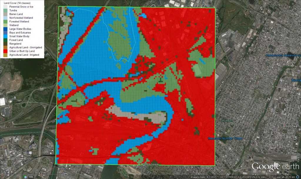
The product should be an ASCII file ready to be imported in the GEO.DAT file. Generating a CSV or Surfer GRD it is possible to make a grid plot for Google Earth (KML here), for example using GEPlot.
This is the Google Earth view of the domain:

And this is the derived Land Cover for CALMET:
